Auto what what now?
AutoGluon is a very capable open-source machine learning package developed by Amazon. It can create predictive ML models for tabular data, time-series, and images. It’s a Python package with a relatively user-friendly interface that makes it easy to build models even if you are not a Python expert (I am not). It has default presets that are easy to use and plenty of options for more advanced users to fine-tune.
Time-series forecasting is a significant chunk of my work so I was curious to explore how well AG performs at this task. AG is very much a “data science” package, designed for working with large datasets and producing forecasts at scale. For time-series forecasting, it includes some “deep learning” or neural-network models like DeepAR as well as standard statistical methods like ARIMA and ETS.
One of AG’s standout features is to produce ensemble models where forecasts are essentially weighted averages of forecasts produced by two or more base models. This allows forecasts from standard statistical models and deep learning models to be combined to potentially perform better than either approach alone. The weights are chosen automatically by AG as part of the model fitting process to optimise forecast accuracy (you can also turn ensembles off if you want to).
Another important feature of AG is that it produces probabalistic forecasts. It gives a distribution of forecast outcomes at each point in time. The default is forecast quantiles from 10% to 90%, although this can be changed. You also get a standard point (mean) forecast.
It can also do fairly sophisticated back-testing (or cross-validation in a time-series context) to help evaluate models and to guide model selection.
Econometrics has entered the chat
My background in forecasting is based on more “traditional” statistical or econometric methods, i.e. time-series regression models and pure time-series models like ARIMA. Way back in the day I did my Masters dissertation on ARIMA forecasting with Peter Phillips and got a good schooling in issues like non-stationarity and cointegration.
In much of my consulting work, forecasting projects often involve only a handful of data series, each with dozens or maybe hundreds of historic data points to base forecasts on. In contrast, in typical a “data science” setting, a large number of forecasts are needed and a lot of effort will be spent on managing data and integrating the forecast outputs with other systems. In that context, individual forecasts are subject to less scrutiny and the emphasis is on the performance and scalability of the system as a whole. In my type of “consulting” context, there is a lot more scrutiny of a much smaller number of forecasts. Working with smaller data also means more scope to build bespoke time-series regression models, rather than solely relying on automated ML approaches.
My clients also often want to know why the forecasts are what they are, and they sometimes want to play what if to test different scenarios. In its current form, AG is more of a black box where forecasts are hard to explain and scenario analysis is not straightforward. This is totally fine in some contexts. In other contexts, “hand building” models based on simple regression or time-series models may be preferable, if the forecasts need to be easily explainable and need individual fine-tuning. There’s no best solution for all contexts, and so it’s great to have more options like AG.
Ok but what about accuracy?
At the end of the day, accuracy of forecasts is one of the most critical factors in choosing a forecasting method. I want to spend the rest of this post discussing a paper by Oleksandr Shchur et al from August 2023 that evaluates the accuracy of AG versus other methods. They did this by comparing forecasts from AG with other methods, for 29 different public datasets of varying sizes and characteristics (note in some of the analysis below I’ve excluded the “COVID deaths” dataset as the forecasts from all models for this dataset were substantially less accurate than all other datasets). My analysis below is based on the tables in their paper and summary data published in the accompanying GitHub repo.
The authors compare AG against standard statistical models and a few other deep learning approaches. Given my background, I’m most interested in the relative benefits of deep learning models compared to the tried and trusty statistical methods. With deep learning methods, we lose explanability of the forecasts and training the models can take a lot more time, but that might be acceptable if the forecasts are more accurate.
Datasets
The following table from the paper summarises the time-series datasets they used. Many are from the M forecasting competitions. Data frequencies vary from hourly to yearly, and dataset sizes range from thousands to millions of data points in total. The number of individual data series in each dataset that are forecast range from dozens to over 145,000.
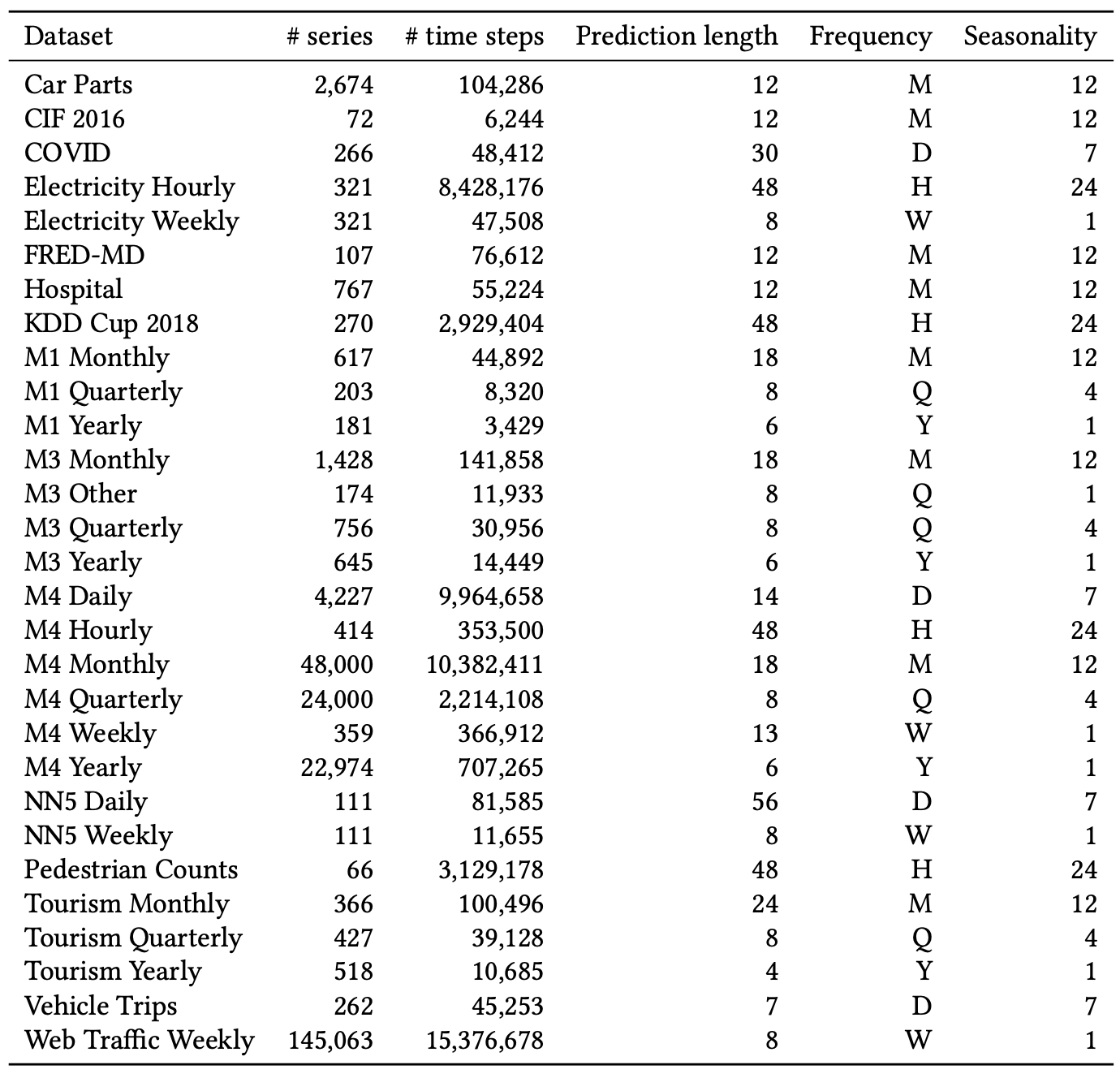
Datasets used in the accuracy tests, from Shchur et al (2023).
The chart below (made by me from the numbers in the table above) shows the average number of data points per data series in each dataset, grouped by the frequencies (note the x-axis is a log scale). Most of the monthly, quarterly, and yearly datasets are similar to the types of data that I most often work with, having fewer than 100 data points per series. Some of the weekly, daily and hourly datasets are much richer with thousands of points per series.
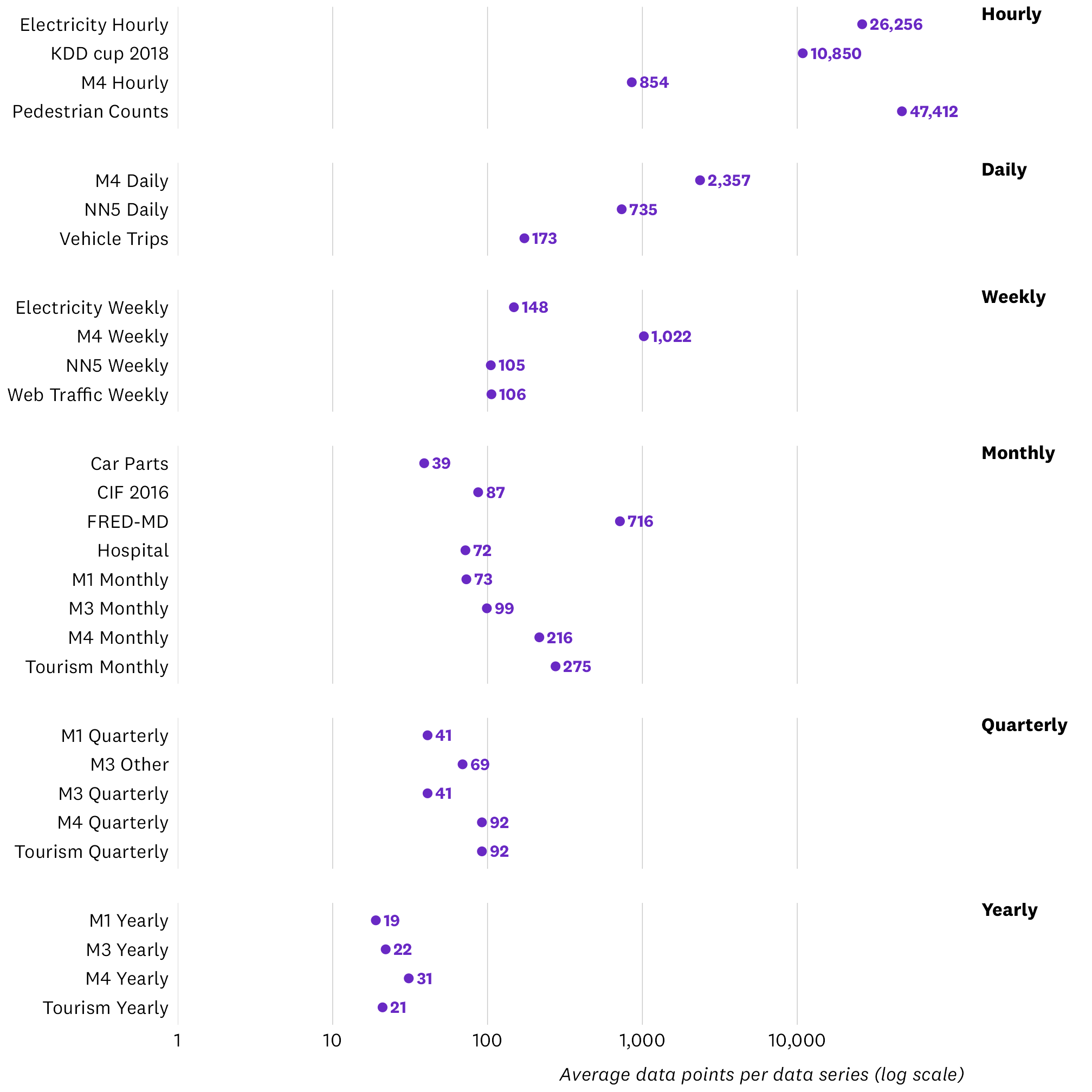
Average number of data points per data series, by dataset.
Forecasting methods compared
The paper tests several different types of models. Accuracy of point forecasts is evaluated using the mean absolute scaled error (MASE). MASE is scale-invariant, so it can be compared across datasets with different scales. Accuracy of forecast distributions is assessed using WQL. In my discussion below, I’ve just focussed on point forecast accuracy (MASE).
The following table from the paper summarises the point accuracy results in terms of the MASE value for each method tested against each dataset (lower MASE is better). The deep learning models are not deterministic (i.e. they can give different forecasts each time they are run with the same training data) so these were run 5 times and the results averaged; the small numbers in brackets are the standard deviation of MASE in those cases. AG performs best among these models for 19 out of the 29 datasets.
This is impressive, but it’s important to note that AG embeds all of the other models except AutoPyTorch (and AG includes some other models not shown in this table). Via its ensembling process, AG will give more weight to models that are more accurate, so it will tend to match the best of the base models in most cases. Across the 19 datasets where AG came out on top, it offered about a 5% improvement in MASE over the second best model, although there are a couple of datasets where it was about 20% better.
Also relevant are the “d.n.f.” results that occur for some of the statistical models. This is where the models did not produce forecasts within six hours (on a fairly powerful 16-core cloud server). That happened for the three datasets that had tens of thousands of data points per data series. Models like ARIMA are not well suited for such long data series, but AG managed to produce a forecast in every case.
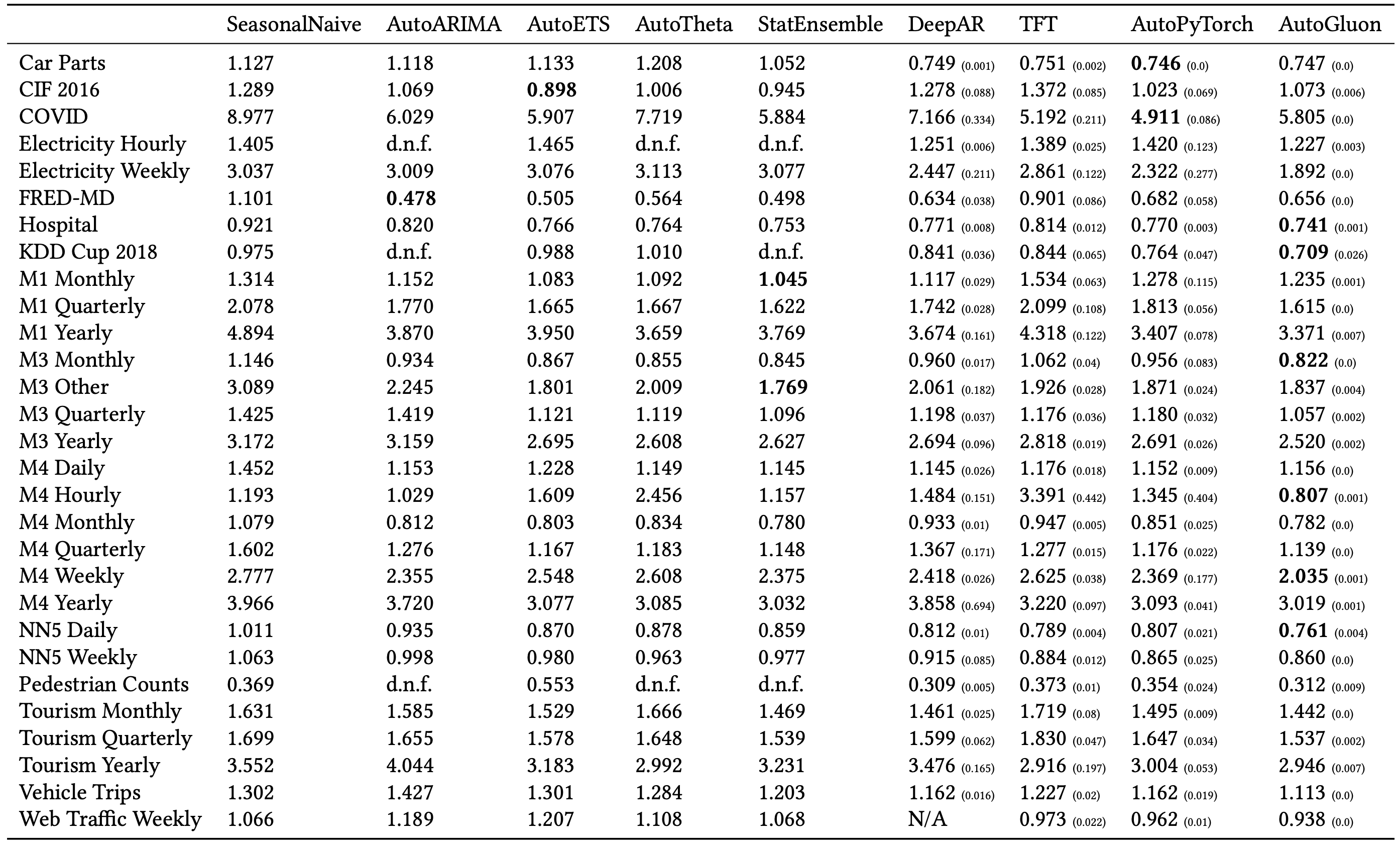
Point accuracy results, from Shchur et al (2023).
Stats models vs deep learning
To take a closer look at the relative benefits of deep learning models, I focussed on three of the forecasting approaches used in the paper:
- StatEnsemble (in the table above): This is a simple ensemble of the AutoARIMA, AutoETS, and AutoTheta models (standard statistical time-series models). The ensemble forecast is just the median of the three forecasts from these models.
- AG best quality (‘AutoGluon’, in the table above): The forecast produced by AG with its “best quality” preset. This involves training a variety of statistical and deep learning models (including those in the table above), and then creating an ensemble forecast of all of them. Ensemble weights are chosen to optimise the forecast accuracy against the training data.
- AG without deep learning (not shown in the table above, but included in the detailed results in the paper’s appendix): This is a restricted version of AG that excludes all the deep learning models. It includes the three statistical models in StatsEnsemble, as well as some other ’tabular’ models that are re-purposed for time-series forecasting. It is also an ensemble approach, with optimised weights.
Of these methods, StatsEnsemble is a standard statistical approach that is fairly easy to implement and trains very quickly on small to medium sized datasets, but may be extremely slow on large datasets. The other two methods include the optimised ensembling benefits of AG, with or without the deep learning models. As above, I wanted to focus on the relative benefits from adding deep learning models into the mix. There might also be some benefit from AG’s approach to finding optimised ensemble weights.
It’s also worth noting that StatsEnsemble forecasts each data series in each dataset in isolation. In contrast the deep learning and ’tabular’ models included in the AG approaches take the dataset as a whole, and thus may be able to exploit relationships that exist among data series to improve the accuracy of forecasts. This is also possible in a statistical model using a vector autoregression, but that type of model wasn’t tested and isn’t currently implemented in AG as far as I can tell.
I created data from the chart below using the point forecast accuracy results from the paper for these three methods. We can see that the AG best quality method has the best accuracy (lowest MASE) in many cases, but in most cases the no deep learning and StatsEnsemble methods are very close behind. There are a few cases where AG best quality performs substantially better than the other methods (eg Electricity Weekly, Car Parts, and M1 Yearly). There are also a few cases where StatsEnsemble is best (eg FRED-MD and M1 Monthly). Note also that StatsEnsemble failed to produce results in three out of the four hourly datasets as explained above.
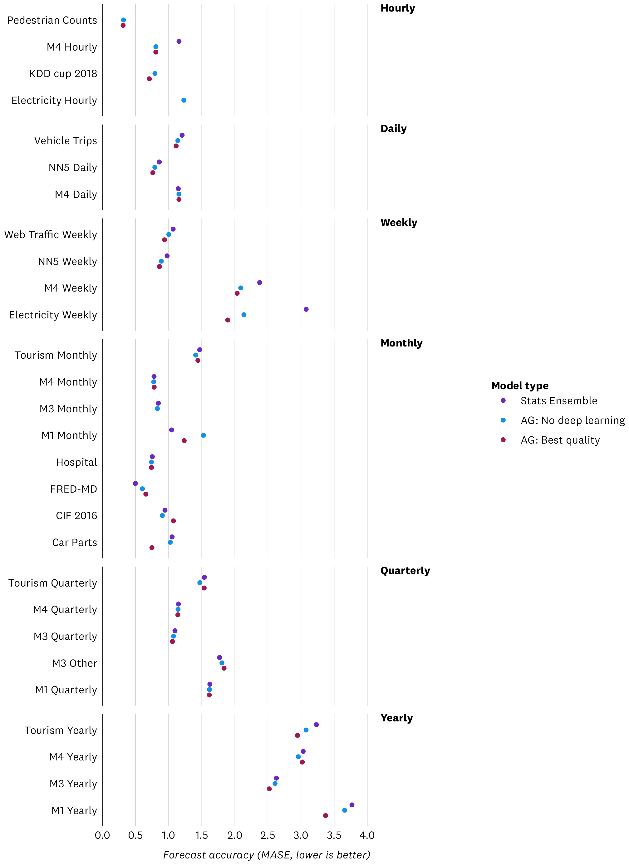
Point forecasting accuracy comparison of selected methods.
Big data vs small data
At the outset, I had a hunch (or bias?) that the deep learning approaches might work better on the larger datasets, but they might suffer from over-fitting and work less well than the simpler statistical methods on smaller datasets. To check this, the chart below compares point forecast accuracy of the AG best quality method with the StatsEnsemble method (the chart shows the difference in MASE across these two methods, for each dataset). As above there are a few cases where AG best quality is much better (the big one is the Electricity Weekly dataset) but smaller differences in most cases.
Interestingly, for the dataset with the largest number of points per data series (M4 Daily, with 2,357 points per series), StatsEnsemble performs fractionally better, but there’s almost nothing in it. So it’s not always the case that deep learning is better with longer data series. However, as above, the stats ensemble models failed to produce any forecasts for the datasets with the very longest data series (Electricity Hourly, KDD cup 2018, and Pedestrian Counts).
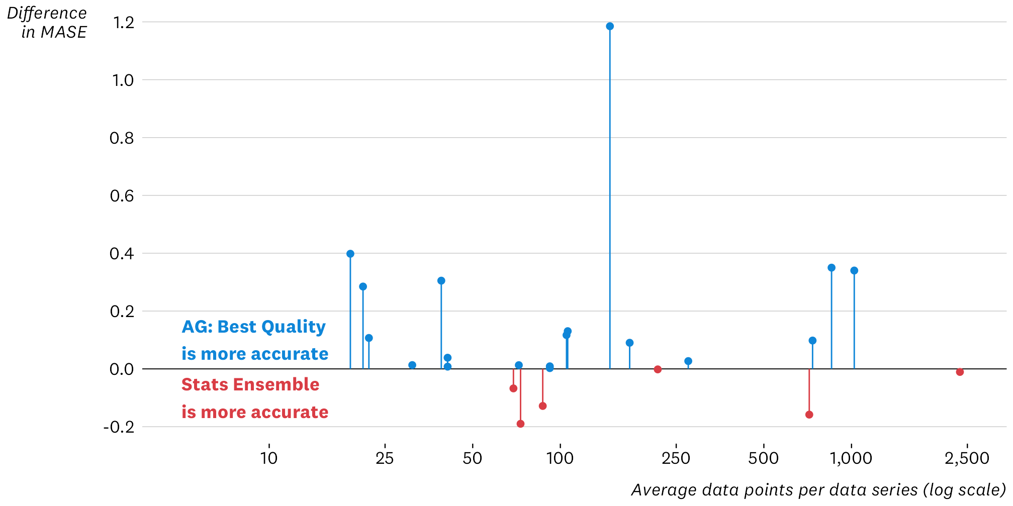
Relative forecasting accuracy of AG best quality vs StatsEnsemble forecasts by average number of data points per data series.
What about the overall size of each dataset? This might matter for the deep learning methods, since they use the full dataset to make predictions, while the stats models use each data series in isolation. The chart below shows the comparison between AG best quality and StatsEnsemble against the total size of each dataset. Again, the StatsEnsemble approach is fractionally better or fractionally worse than AG best quality for some of the largest datasets, including M4 Monthly and M4 Daily with around 10 million data points each.
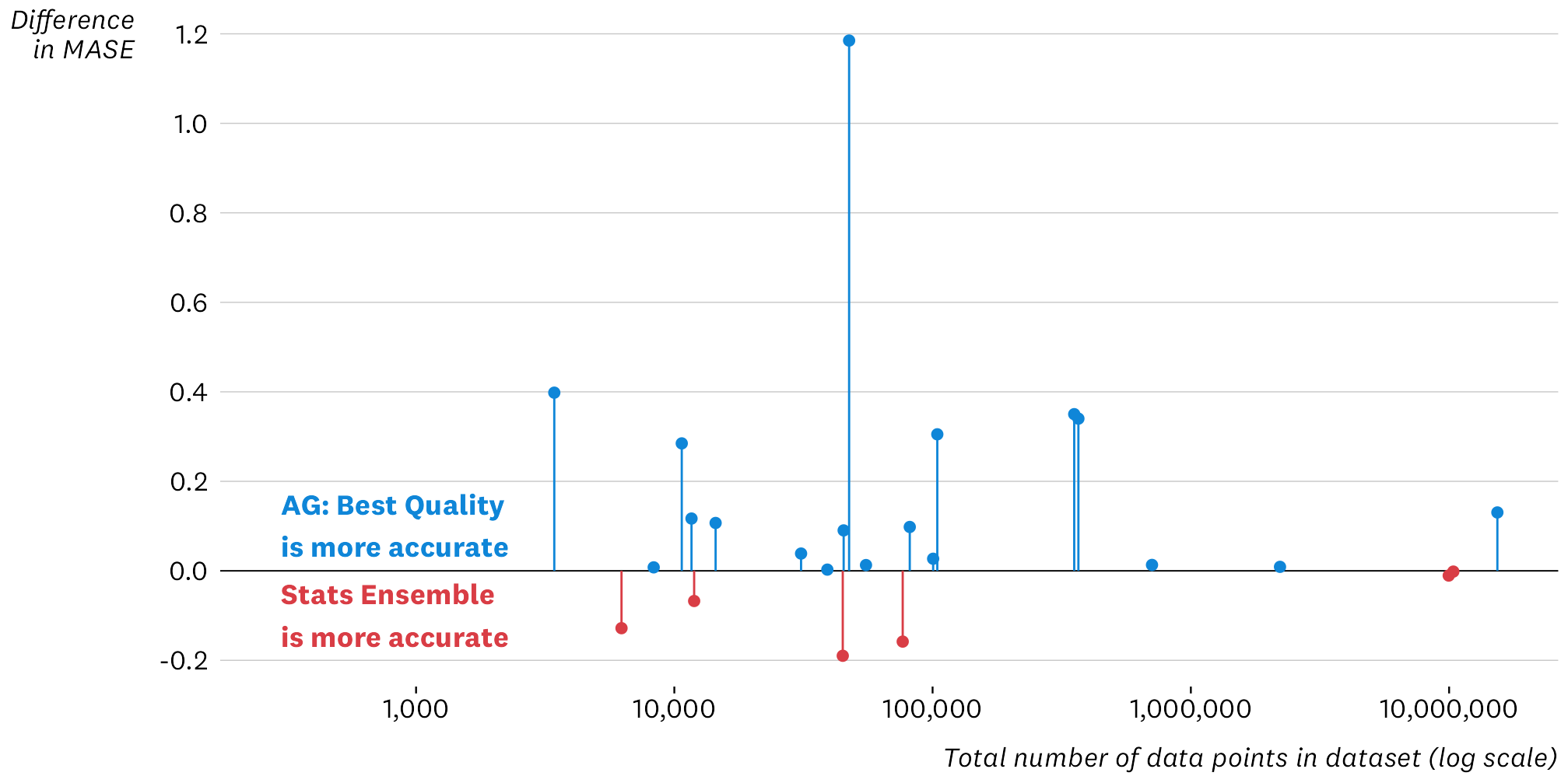
Relative forecasting accuracy of AG best quality vs StatsEnsemble forecasts by total number of data points in each dataset.
So, contrary to my initial expectation, it doesn’t seem like longer data series or longer datasets make deep learning forecasts more accurate. Instead the differences probably come from other characteristics of the data, such as the strength of correlations across data series within a dataset.
Conclusions
My main conclusions from this are:
- AG offers substantial improvements in forecast accuracy over traditional statistical forecasting models in certain cases, but it’s not universally better.
- When AG is worse than statistical methods, it’s not worse by very much. It seems like using AG doesn’t involve a big risk of much less accurate point forecasts than simpler methods. I guess this is not surprising since AG embeds these methods and will pick them up in its ensemble forecasts if indeed they are accurate.
- In a lot of cases, statistical methods are also fine, particularly if you take a simple ensemble of basic models like ARIMA and ETS, as done in the StatsEnsemble example above.
- Some of the benefits of AG come from its optimised approach to ensembling and overall ease of use. You can always turn off the deep learning models and use simpler models in the ensemble. This should give models that train quickly and are reasonably accurate in most cases.
Horses for courses
So am I going to use AG for my forecasting work? Yes, in the right context, and it’s always good to have more tools in the toolbox. If I need to produce quick and reasonably accurate forecasts, I’ll probably avoid deep learning and stick to a simple ensemble of statistical models. AG looks like a convenient way to implement this, even with my limited python skills. If I need to produce many forecasts for a large and complicated dataset, deep learning methods might have advantages that justify the extra time and cost involved, and loss of explainability. If I need a highly transparent, explainable model that can be used for scenario analysis, I’m probably still going to want a traditional time-series regression model.